One GUI, many engines
ProMOST sizes one transistor at a time, using your PDK's own compact model, in real time. The main GUI does the dimensioning; add-ins take the same device into distortion, RF, switched configurations, the full W–L plane, your design suite and your Python scripts. Nothing is re-entered, and there is no "Run" button to wait for.
The main GUI at the centre,
capabilities all around it
Every add-in inherits the device, bias point and sweep setup from the main GUI, and runs on the same solvers. Click one to see what it computes.
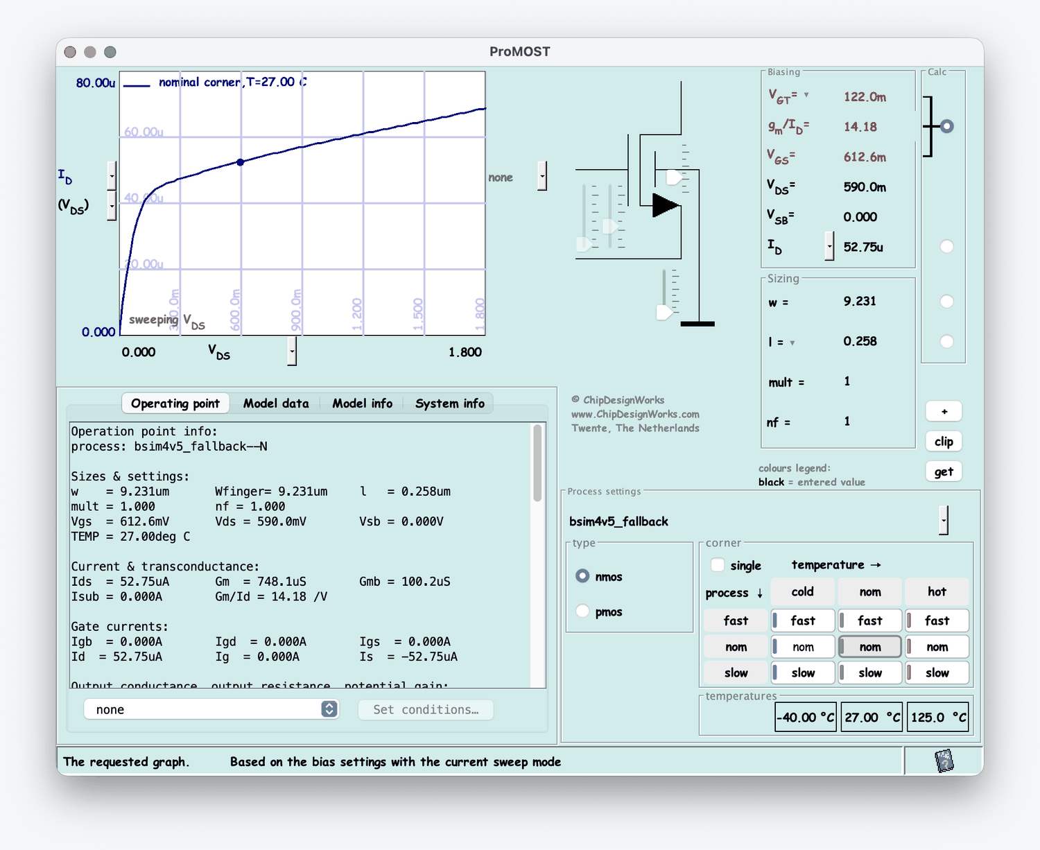
- Solve for whichever parameter you don't know: W, L, ID/gm, or the {VGS, VGT, gm/ID} set
- Basic and constrained sweeps, plotted against VGS, VGT, gm/ID or the inversion coefficient
- Full OP report: DC, small-signal, noise, spread/mismatch, loaded y- and s-parameters
- 3×3 corner grid with editable temperatures, overlaid in a single graph
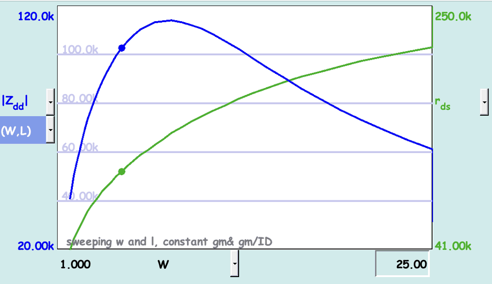
The main GUI sweeps W or L at constant ID or gm. This add-in sweeps both, giving a colour map of any parameter across the entire W–L plane with your specifications applied as a filter.
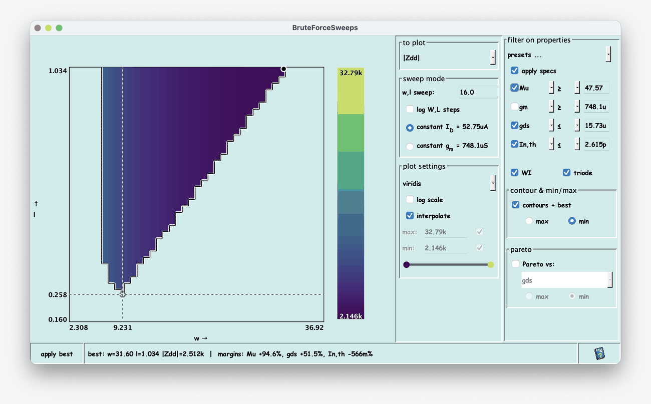
- Plot any OP parameter (|Zdd|, gds, µ, noise) over W and L at constant ID or gm
- Filter on properties (with presets) greys out every sizing that fails your specs, drawing the feasible design region
- Contours + best marks the optimum; Pareto vs: overlays the trade-off front between two parameters
- Apply best pushes the recommended W and L straight into the main GUI, with the margin on each spec
Non-linearity of the real device, computed by a quasi-PSS engine rather than a fitted polynomial. Sweep it exactly like a DC sweep and read the sweet spot off the graph.
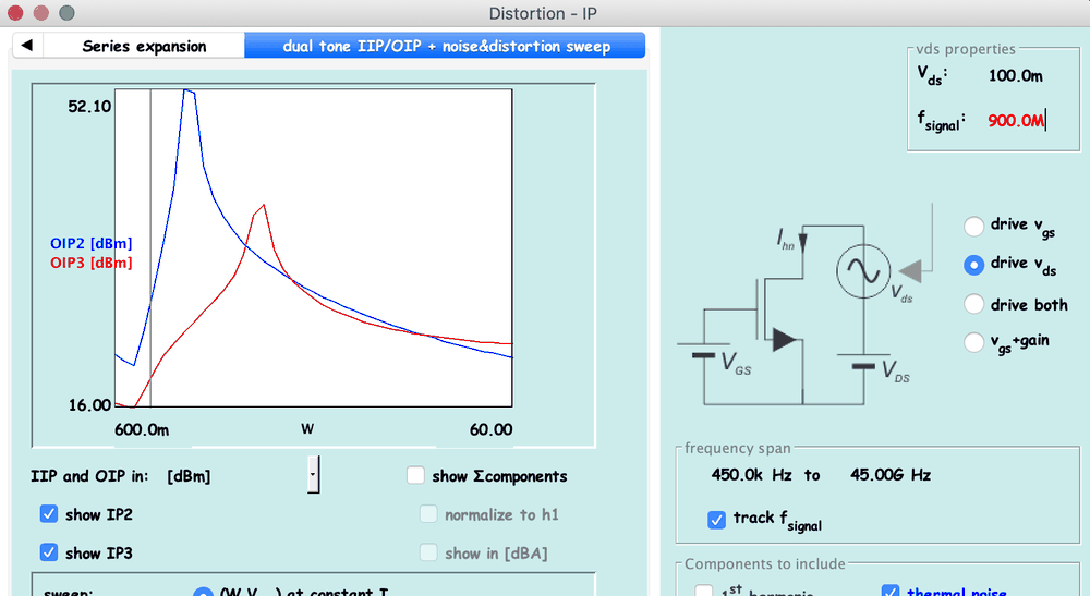
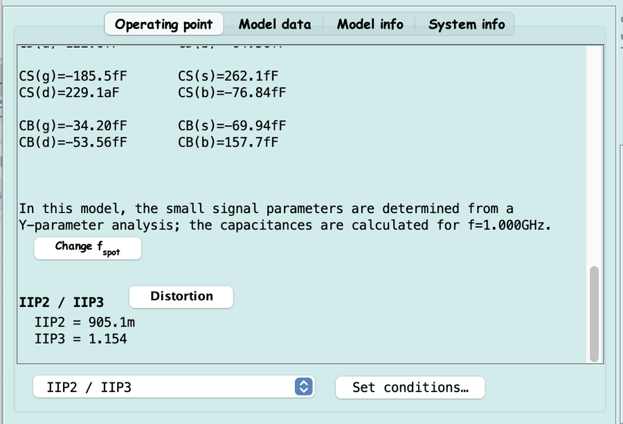
- Spectra with harmonics and noise; IP2/IP3, input- and output-referred, over constrained sweeps
- Analytic Taylor/Volterra 2-port expansion coefficients, which stay reliable near a sweet spot, where an FFT disappears into its own noise floor
- An nth-order Verilog-A model generator, to pin down where the non-linearity comes from
- Headline outputs such as IIP3 can be pinned into the main OP pane, with a warning when a value approaches the noise floor
The same device and the same constrained sweep, now inside its embedding network. The device comes from the main GUI; you add the terminations around it.
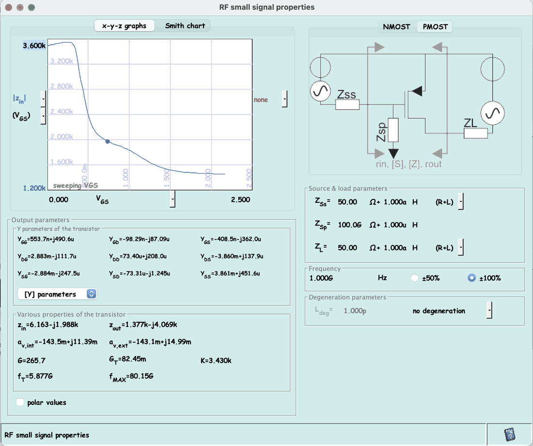
- Y-, Z- and S-parameters, zin, zout, G, GT, av, fT, fmax and stability factors
- Set ZSs, ZSp, ZL and inductive source degeneration, so the numbers describe your actual stage instead of a bare device
- Plot on x-y-z axes or on a Smith chart; sweep VGS, VDS, frequency, temperature, or (VGS,W)/(VGS,L) at constant ID or gm
- Export S-parameters to Touchstone, and cross-check the result against Spectre
The main GUI assumes a common-source device, which real circuits frequently are not. This add-in biases and evaluates the transistor in the configuration you actually built.
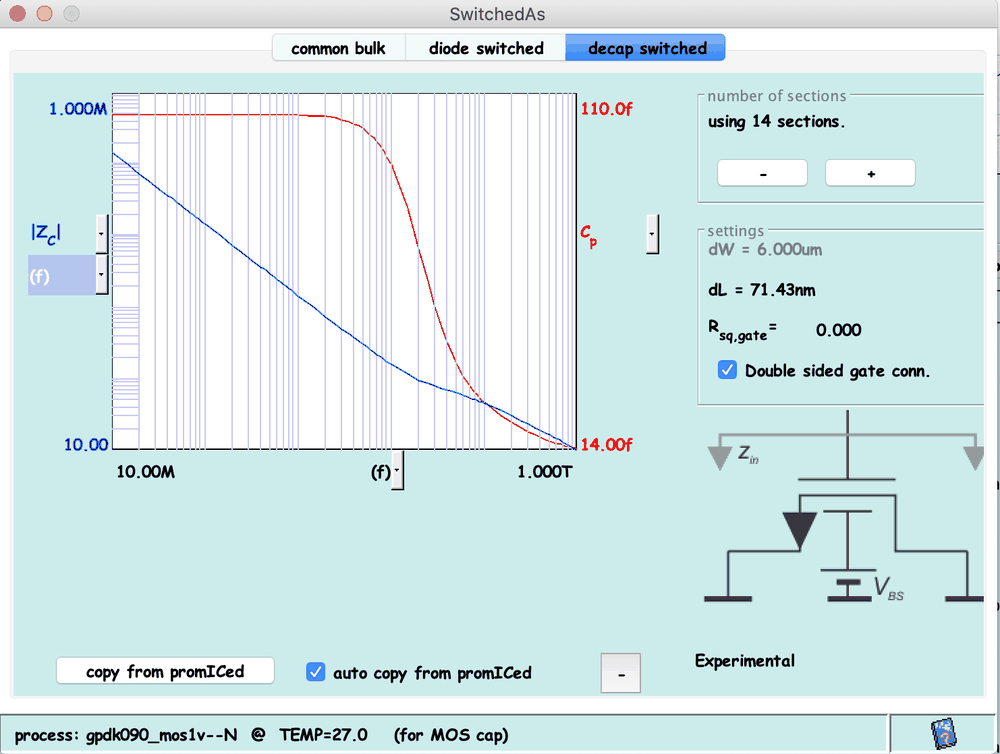
- Diode-switched, common-gate and MOS-capacitor configurations
- Decap-switched MOS: equivalent impedance and capacitance as a function of frequency
- Lumped non-quasi-static equivalents, so a decap's loss is visible long before layout
- Same process, corner and temperature settings as the main GUI
ProMOST is a MOS tool, but BiCMOS designs need their bipolar devices dimensioned too, in the same session and in the same way.
- Mextram-based operating point for NPN and PNP devices
- Noise, S-parameters and stability analysis
- The same sweep-and-read workflow as the MOS side of the tool
- Uses the bipolar model data from your converted PDK
The reverse direction: take the accurate device and derive the simple model, with every coefficient carrying a textbook meaning (β, VTH, λ, Cox), fitted at your operating point, in your technology.
- Square-law and simplified-EKV equivalents of the live device, regenerated automatically as you change the bias point
- Output as a ready-to-use Verilog-A module, a Mathematica fragment with plots, and an Excel workbook
- The workbook compares the idealized model against the full ProMOST model over VDS and VGS sweeps, so you can see exactly where they deviate
- Made for teaching and for hand analysis: the square law next to a real short-channel device
ProMOST as a calculation engine behind your own script, over a pipe or a socket, with Python, MATLAB or a Jupyter notebook on the other end.
# one setup line, then one line per sweep point
setup = "format=value;isn=true;l=0.5;vds=0.6;gm=10e-3;calcvgtvgs"
# W sweeps; VGS is re-solved at every point to hold gm on target
for w in widths:
    vgs, id_, oip3 = promost(f"w={w};vgs=?;id=?;OIP(1e9)=?")
- Select devices, set bias and sizing, run constrained sweeps, read OP, RF and IIP/OIP data
- Parameter studies and technology comparisons become scripts you rerun on every PDK update
- Feed results into your own optimizers, notebooks or regression suites
- Python and MATLAB examples ship with the distribution
Select a device on your schematic, size it in ProMOST and push the result back: a full round trip, not just an export.
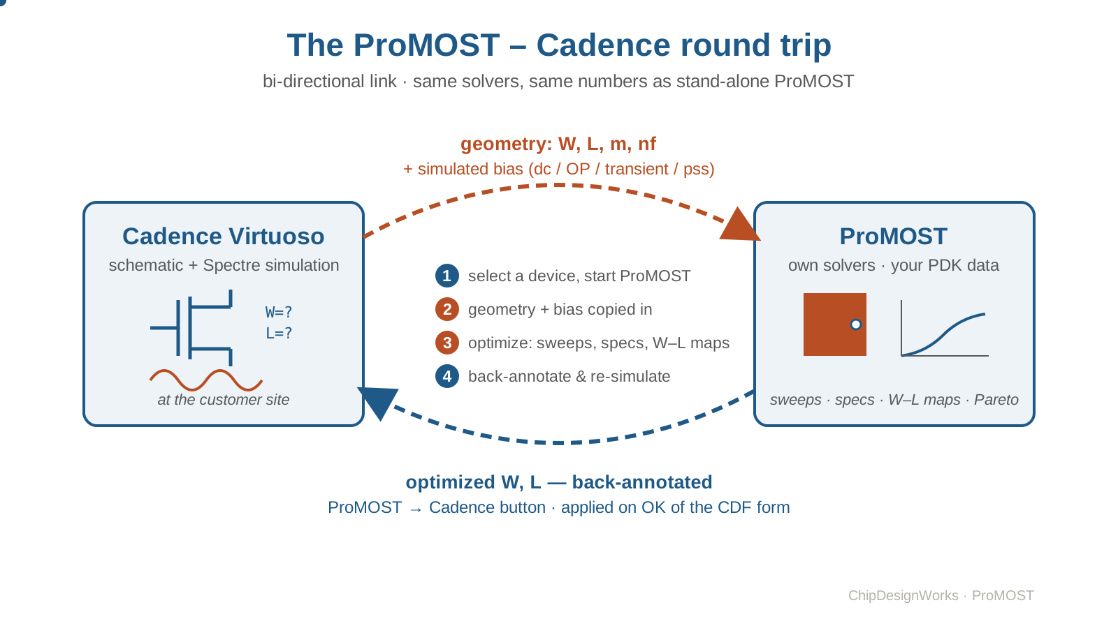
- Start from the instance menu or a bindkey; W, L, m and nf are copied automatically
- Process match and type match indicators confirm you are looking at the same device
- Load the bias point from dc, OP, tran or td-pss simulation data, with a slider that walks along the sweep variable or along time
- Optimize, then push the new geometry back into the schematic
Click an add-in to see what it computes, or go
Solve for the parameter
you do not know
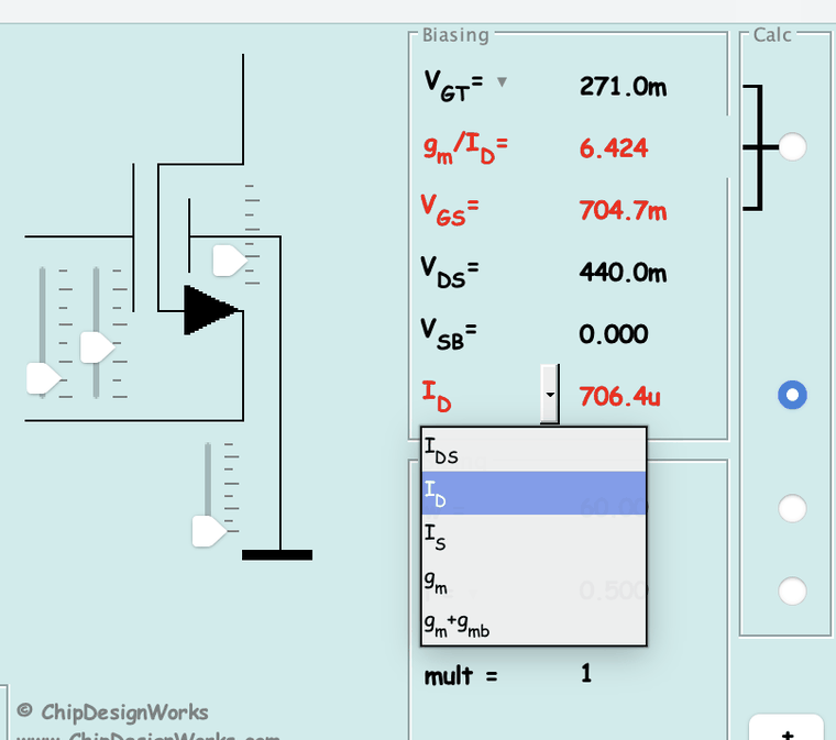
A designer rarely knows W. They know the gm they need, the current they can spend, and the length that buys enough output impedance. ProMOST lets you mark any one parameter as free and solves it from all the others, instantly, from the real compact model.
"Give me the L that delivers gm = 5 mS at VGT = 150 mV, VDS = 0.6 V and W = 20 µm" is answered in well under a second. Entered values are shown in black and solved values in red, so the input/output split is never in doubt.
- No "Run" button. Every edit, including every release of a bias slider, triggers a recalculation, typically well under a second, even for compound models.
- Sliders on every bias field. Drag VGS on the transistor symbol and watch the operating point move.
- Auto-stacking with a preferred length for series devices, set from the sizing pane.
- Manual recalculation is one setting away for heavy multi-dimensional work.
Sweeps that hold
your design constraint
An unconstrained W sweep changes the current along with the width, which is rarely the question you are asking. ProMOST's constrained sweeps hold ID or gm fixed and re-solve VGS as they go, giving the trade-off curve you actually design against.
See the device
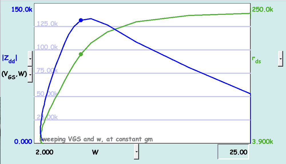
Sweep VDS, VGS, W, L or temperature. Plot any OP parameter on either y-axis and any OP parameter on the x-axis, linear or logarithmic, two curves at a time.
Design the device
(VGS,W), (VGS,L) and (VGS,T) at constant ID or gm; W and L at constant active area or at constant scale. The graph states which quantity is held, and at what value.
Your methodology
Put gm/ID, VGT or the inversion coefficient on the x-axis and the plots become standard gm/ID design charts. Make it the default and ProMOST opens that way, every time.
Everything a designer
reads from an OP
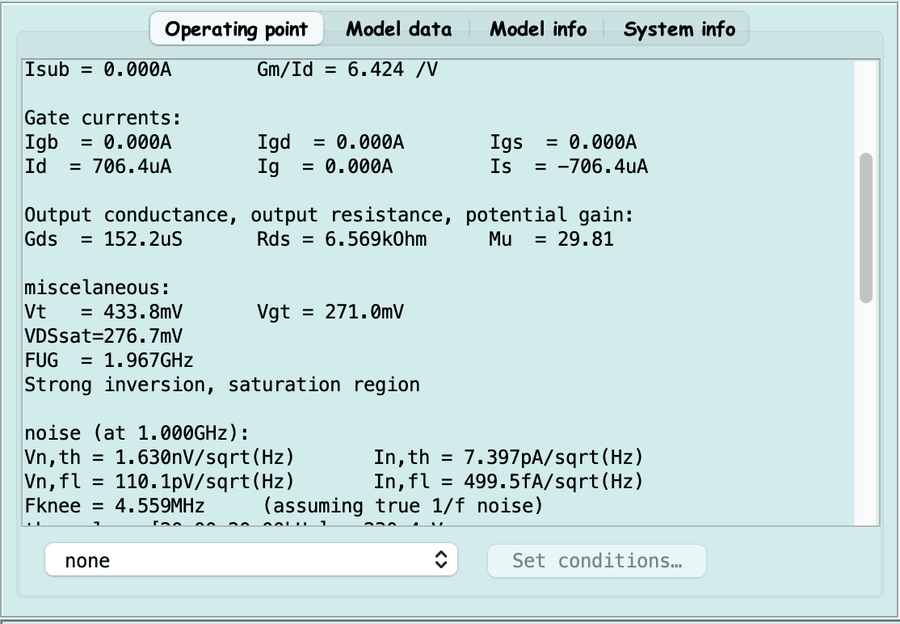
ProMOST's own op, dc, ac and noise solvers run the full compact model, including everything the PDK wraps around it. What ProMOST reports is what your simulator will report.
- Large- and small-signal OP: currents, transconductances, output conductance, capacitances, potential gain, operating region
- Noise: input- and output-referred, at a spot frequency or integrated over a band you set
- Spread and mismatch of IDS and of the overdrive voltage, before you commit to an area
- Loaded y- and s-parameters, with small-signal parameters optionally taken from the y-parameter run
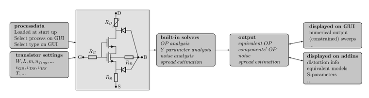
- Compound models: per-component OP data for every transistor, diode, juncap, passive and Verilog-A block, plus the equivalent OP of the complete device
- Equivalent circuits generated from the operating point
- Add-in results pinned in: select e.g. IIP2/IIP3 in the picker and it is appended below the OP data, together with its evaluation conditions
- Export: graphs and data to XLS, CSV or TikZ, straight into your report
Corners and temperature,
before you commit
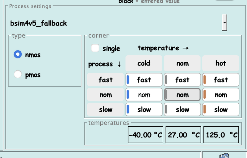
A size that only works at nominal is not a usable size. The process pane holds a 3×3 selector, {fast, nom, slow} × {cold, nom, hot}, and sweeps can be overlaid for several corners in one graph, so the spread of gm, fT or noise is visible while you are still choosing W and L.
- All three temperatures are editable: type your own −40 °C, 27 °C, 125 °C, or anything else
- Process corners are available wherever your converted PDK provides corner data
- The (VGS,T) constrained sweep shows the VGS range a constant-gm pair needs across temperature
Your PDK's models,
run as they are
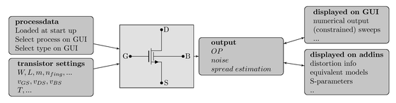
ProMOST does not fit a surrogate. It runs the compact model from your PDK in its own background solvers, on the complete subcircuit, which is why its answers hold up once you reach the simulator.
Solved as one device
Transistors wrapped in subcircuits with diodes, juncaps and passives are solved whole, with per-component OP data and the equivalent OP of the complete model.
op · dc · ac · noise · quasi-PSS
ProMOST ships its own DC, AC, noise and quasi-PSS solvers and runs stand-alone, so no external simulator is involved while you dimension.
Once per PDK release
Import Spectre or (H)SPICE process data through reusable recipe files. A run takes minutes, is done once by CAD support and is shared by the whole group. ConversionVerifier regression-tests the result.
Finding the right sweep
without reading the manual
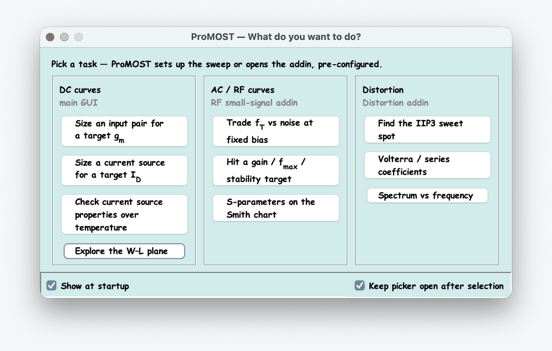
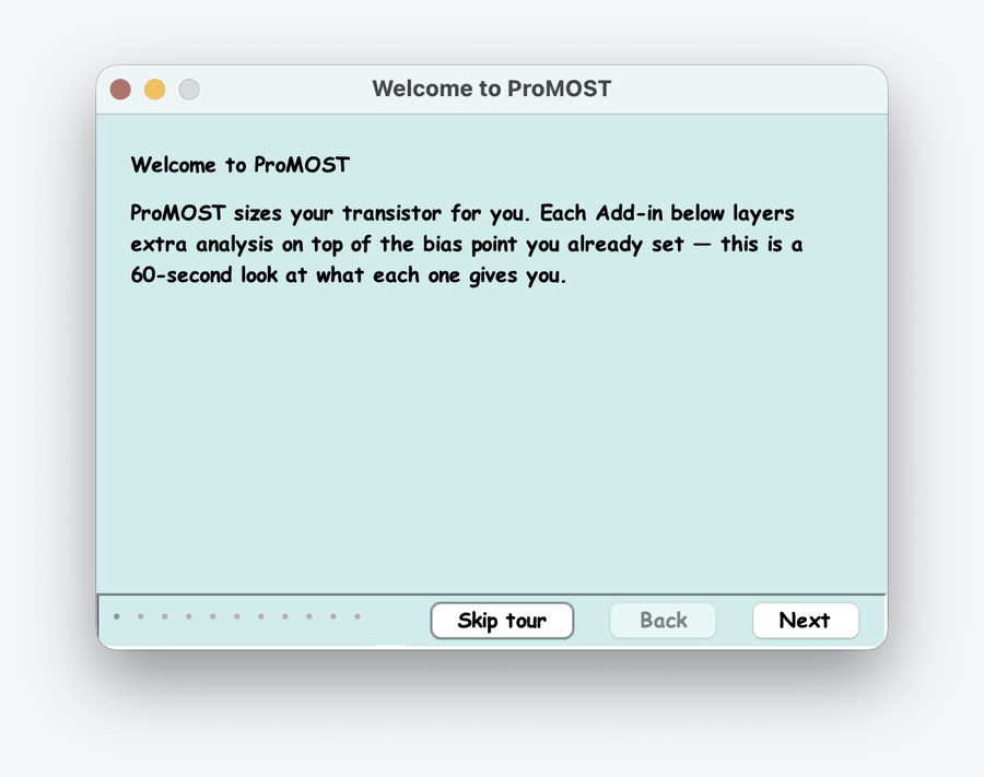
ProMOST has more sweep modes and add-in outputs than anyone discovers by clicking around. Two built-in guides close that gap.
Getting started is
a one-afternoon job
Linux & macOS
macOS on Apple Silicon and Intel; multiple Linux flavours. Node-locked or RLM floating licences, with per-group and per-user customization. Requires a Java runtime 1.8 or higher.
Recipe files
TheConverter turns Spectre/HSPICE process data into ProMOST technology files. Written once per PDK release, then reused by everyone in the group.
However you work
Stand-alone, embedded in your design suite through the integration add-in, or driven from Python and MATLAB through TheRemote.
In use at electronics companies, design houses and universities worldwide.